1 Presentation
This is the multivariate analysis code for the paper “Changes in Beliefs about Meritocracy and Preferences for Market Justice in the Chilean School Context”. The prepared data is edumer_students_long.RData.
2 Libraries
3 Data
Show the code
load(file = here("output/data/db_proc.RData"))

glimpse(db_proc)
Rows: 1,156
Columns: 23
$ id_student <dbl> 191617388, 191617388, 191617613, 191617613, 19164733…
$ wave <fct> 1, 2, 1, 2, 1, 2, 1, 2, 1, 2, 1, 2, 1, 2, 1, 2, 1, 2…
$ curse_level <fct> 6to, 7mo, 1ro, 2do, 6to, 7mo, 6to, 7mo, 6to, 7mo, 6t…
$ perc_effort <dbl> 3, 2, 3, 3, 4, 2, 3, 3, 2, 2, 3, 3, 3, 4, 4, 2, 3, 2…
$ perc_talent <dbl> 3, 3, 3, 3, 4, 2, 4, 3, 3, 3, 3, 3, 3, 3, 3, 3, 3, 3…
$ perc_rich_parents <dbl> 2, 4, 4, 3, 2, 4, 4, 4, 4, 3, 4, 4, 4, 3, 2, 2, 2, 4…
$ perc_contact <dbl> 3, 4, 4, 3, 3, 4, 4, 4, 3, 2, 4, 3, 3, 3, 3, 2, 4, 3…
$ pref_effort <dbl> 4, 3, 4, 3, 3, 3, 4, 4, 4, 4, 4, 4, 4, 4, 3, 3, 4, 3…
$ pref_talent <dbl> 3, 2, 3, 3, 2, 2, 2, 4, 3, 3, 4, 3, 3, 4, 2, 2, 2, 2…
$ pref_rich_parents <dbl> 2, 2, 4, 2, 2, 2, 2, 2, 3, 4, 2, 2, 3, 2, 2, 2, 2, 2…
$ pref_contact <dbl> 3, 2, 4, 2, 2, 2, 3, 3, 3, 3, 2, 2, 3, 2, 3, 3, 3, 4…
$ school_effort <dbl> 4, 3, 3, 3, 4, 3, 3, 3, 4, 4, 3, 3, 3, 4, 3, 3, 3, 4…
$ school_talent <dbl> 4, 3, 3, 3, 4, 3, 3, 3, 4, 3, 4, 4, 3, 3, 2, 2, 4, 4…
$ just_educ <dbl> 3, 2, 3, 3, 2, 1, 1, 2, 4, 1, 2, 3, 3, 4, 2, 2, 3, 2…
$ just_health <dbl> 3, 2, 2, 2, 2, 1, 1, 1, 4, 1, 2, 3, 2, 1, 1, 1, 1, 1…
$ just_pension <dbl> 2, 2, 2, 2, 4, 1, 1, 1, 4, 1, 1, 2, 3, 1, 3, 2, 1, 1…
$ gender <fct> Male, Male, Female, Female, Male, Other, Female, Fem…
$ age <dbl> 13, 13, 17, 17, 13, 13, 12, 12, 13, 13, 13, 13, 13, …
$ books <fct> Less than 25, Less than 25, Less than 25, Less than …
$ cohort_level <fct> Primary, Primary, Secondary, Secondary, Primary, Pri…
$ mjp <dbl> 2.666667, 2.000000, 2.333333, 2.333333, 2.666667, 1.…
$ age2 <dbl> 169, 169, 289, 289, 169, 169, 144, 144, 169, 169, 16…
$ parental_educ <fct> Technical higher education, Technical higher educati…4 Analysis
4.1 Descriptives
Data Frame Summary
db_proc
Dimensions: 1156 x 23Duplicates: 0
| No | Variable | Label | Stats / Values | Freqs (% of Valid) | Graph | Valid | Missing | ||||||||||||||||||||||||||||||||||||||||||||||||||||||||||||||||||||||
|---|---|---|---|---|---|---|---|---|---|---|---|---|---|---|---|---|---|---|---|---|---|---|---|---|---|---|---|---|---|---|---|---|---|---|---|---|---|---|---|---|---|---|---|---|---|---|---|---|---|---|---|---|---|---|---|---|---|---|---|---|---|---|---|---|---|---|---|---|---|---|---|---|---|---|---|---|---|
| 1 | id_student [numeric] | Unique student identifier |
|
578 distinct values |  |
1156 (100.0%) | 0 (0.0%) | ||||||||||||||||||||||||||||||||||||||||||||||||||||||||||||||||||||||
| 2 | wave [factor] | Wave |
|
|
 |
1156 (100.0%) | 0 (0.0%) | ||||||||||||||||||||||||||||||||||||||||||||||||||||||||||||||||||||||
| 3 | curse_level [factor] | Student level |
|
|
 |
1156 (100.0%) | 0 (0.0%) | ||||||||||||||||||||||||||||||||||||||||||||||||||||||||||||||||||||||
| 4 | perc_effort [numeric] | In Chile, people are rewarded for their efforts |
|
|
 |
1156 (100.0%) | 0 (0.0%) | ||||||||||||||||||||||||||||||||||||||||||||||||||||||||||||||||||||||
| 5 | perc_talent [numeric] | In Chile, people are rewarded for their intelligence and ability |
|
|
 |
1156 (100.0%) | 0 (0.0%) | ||||||||||||||||||||||||||||||||||||||||||||||||||||||||||||||||||||||
| 6 | perc_rich_parents [numeric] | In Chile, those with wealthy parents fare much better in life |
|
|
 |
1156 (100.0%) | 0 (0.0%) | ||||||||||||||||||||||||||||||||||||||||||||||||||||||||||||||||||||||
| 7 | perc_contact [numeric] | In Chile, those with good contacts do better in life |
|
|
 |
1156 (100.0%) | 0 (0.0%) | ||||||||||||||||||||||||||||||||||||||||||||||||||||||||||||||||||||||
| 8 | pref_effort [numeric] | Those who put in more effort should receive greater rewards than those who put in less effort |
|
|
 |
1156 (100.0%) | 0 (0.0%) | ||||||||||||||||||||||||||||||||||||||||||||||||||||||||||||||||||||||
| 9 | pref_talent [numeric] | Those who have more talent should receive greater rewards than those who have less talent |
|
|
 |
1156 (100.0%) | 0 (0.0%) | ||||||||||||||||||||||||||||||||||||||||||||||||||||||||||||||||||||||
| 10 | pref_rich_parents [numeric] | It’s fine that those whose parents are wealthy do well in life |
|
|
 |
1156 (100.0%) | 0 (0.0%) | ||||||||||||||||||||||||||||||||||||||||||||||||||||||||||||||||||||||
| 11 | pref_contact [numeric] | It’s fine that those who have good connections do well in life |
|
|
 |
1156 (100.0%) | 0 (0.0%) | ||||||||||||||||||||||||||||||||||||||||||||||||||||||||||||||||||||||
| 12 | school_effort [numeric] | In this school, those who put in effort get good grades |
|
|
 |
1156 (100.0%) | 0 (0.0%) | ||||||||||||||||||||||||||||||||||||||||||||||||||||||||||||||||||||||
| 13 | school_talent [numeric] | In this school, those who are intelligent get good grades |
|
|
 |
1156 (100.0%) | 0 (0.0%) | ||||||||||||||||||||||||||||||||||||||||||||||||||||||||||||||||||||||
| 14 | just_educ [numeric] | It’s good that those who can pay more receive a better education |
|
|
 |
1156 (100.0%) | 0 (0.0%) | ||||||||||||||||||||||||||||||||||||||||||||||||||||||||||||||||||||||
| 15 | just_health [numeric] | It’s good that those who can pay more have better access to healthcare |
|
|
 |
1156 (100.0%) | 0 (0.0%) | ||||||||||||||||||||||||||||||||||||||||||||||||||||||||||||||||||||||
| 16 | just_pension [numeric] | It’s good that in Chile, people with higher incomes can have better pensions than those with lower incomes |
|
|
 |
1156 (100.0%) | 0 (0.0%) | ||||||||||||||||||||||||||||||||||||||||||||||||||||||||||||||||||||||
| 17 | gender [factor] | Gender |
|
|
 |
1156 (100.0%) | 0 (0.0%) | ||||||||||||||||||||||||||||||||||||||||||||||||||||||||||||||||||||||
| 18 | age [numeric] | Age |
|
|
 |
1156 (100.0%) | 0 (0.0%) | ||||||||||||||||||||||||||||||||||||||||||||||||||||||||||||||||||||||
| 19 | books [factor] | Books at home |
|
|
 |
1156 (100.0%) | 0 (0.0%) | ||||||||||||||||||||||||||||||||||||||||||||||||||||||||||||||||||||||
| 20 | cohort_level [factor] | Student cohort |
|
|
 |
1156 (100.0%) | 0 (0.0%) | ||||||||||||||||||||||||||||||||||||||||||||||||||||||||||||||||||||||
| 21 | mjp [numeric] | Market Justice Preferences |
|
|
 |
1156 (100.0%) | 0 (0.0%) | ||||||||||||||||||||||||||||||||||||||||||||||||||||||||||||||||||||||
| 22 | age2 [numeric] | Age^2 |
|
|
 |
1156 (100.0%) | 0 (0.0%) | ||||||||||||||||||||||||||||||||||||||||||||||||||||||||||||||||||||||
| 23 | parental_educ [factor] | Parental educational level |
|
|
 |
1156 (100.0%) | 0 (0.0%) | ||||||||||||||||||||||||||||||||||||||||||||||||||||||||||||||||||||||
Generated by summarytools 1.0.1 (R version 4.2.2)
2025-01-27
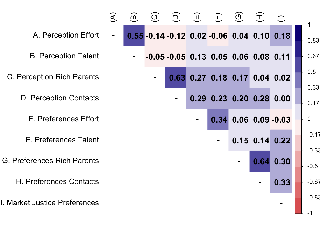
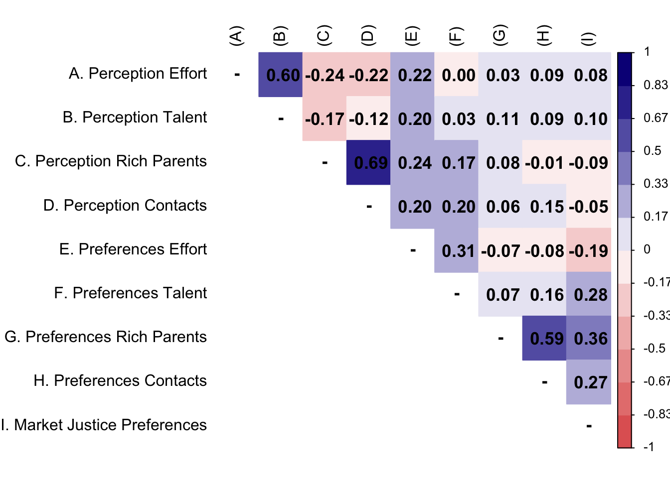
4.2 Measurement model
Show the code
M1 <- psych::polychoric(db_proc[db_proc$wave==1,][c(4:11,21)])

P1 <- cor(db_proc[db_proc$wave==1,][c(4:11,21)], method = "pearson", use = "complete.obs")

diag(M1$rho) <- NA

diag(P1) <- NA

M1$rho[9,] <- P1[9,]

M2 <- psych::polychoric(db_proc[db_proc$wave==2,][c(4:11,21)])

P2 <- cor(db_proc[db_proc$wave==2,][c(4:11,21)], method = "pearson", use = "complete.obs")

diag(M2$rho) <- NA

diag(P2) <- NA

M2$rho[9,] <- P2[9,]

rownames(M1$rho) <- c("A. Perception Effort",
                     "B. Perception Talent",
                     "C. Perception Rich Parents",
                     "D. Perception Contacts",
                     "E. Preferences Effort",
                     "F. Preferences Talent",
                     "G. Preferences Rich Parents",
                     "H. Preferences Contacts",
                     "I. Market Justice Preferences")

#set Column names of the matrix
colnames(M1$rho) <-c("(A)", "(B)","(C)","(D)","(E)","(F)","(G)",
                       "(H)","(I)")

rownames(P1) <- c("A. Perception Effort",
                     "B. Perception Talent",
                     "C. Perception Rich Parents",
                     "D. Perception Contacts",
                     "E. Preferences Effort",
                     "F. Preferences Talent",
                     "G. Preferences Rich Parents",
                     "H. Preferences Contacts",
                     "I. Market Justice Preferences")

#set Column names of the matrix
colnames(P1) <-c("(A)", "(B)","(C)","(D)","(E)","(F)","(G)",
                    "(H)","(I)")


rownames(M2$rho) <- c("A. Perception Effort",
                     "B. Perception Talent",
                     "C. Perception Rich Parents",
                     "D. Perception Contacts",
                     "E. Preferences Effort",
                     "F. Preferences Talent",
                     "G. Preferences Rich Parents",
                     "H. Preferences Contacts",
                     "I. Market Justice Preferences")

#set Column names of the matrix
colnames(M2$rho) <-c("(A)", "(B)","(C)","(D)","(E)","(F)","(G)",
                       "(H)","(I)")

rownames(P2) <- c("A. Perception Effort",
                     "B. Perception Talent",
                     "C. Perception Rich Parents",
                     "D. Perception Contacts",
                     "E. Preferences Effort",
                     "F. Preferences Talent",
                     "G. Preferences Rich Parents",
                     "H. Preferences Contacts",
                     "I. Market Justice Preferences")

#set Column names of the matrix
colnames(P2) <-c("(A)", "(B)","(C)","(D)","(E)","(F)","(G)",
                    "(H)","(I)")
Show the code
corrplot::corrplot(
    M1$rho,
    method = "color",
    type = "upper",
    col = colorRampPalette(c("#E16462", "white", "#0D0887"))(12),
    tl.pos = "lt",
    tl.col = "black",
    addrect = 2,
    rect.col = "black",
    addCoef.col = "black",
    cl.cex = 0.8,
    cl.align.text = 'l',
    number.cex = 1.1,
    na.label = "-",
    bg = "white"
  )
Show the code
corrplot::corrplot(
    M2$rho,
    method = "color",
    type = "upper",
    col = colorRampPalette(c("#E16462", "white", "#0D0887"))(12),
    tl.pos = "lt",
    tl.col = "black",
    addrect = 2,
    rect.col = "black",
    addCoef.col = "black",
    cl.cex = 0.8,
    cl.align.text = 'l',
    number.cex = 1.1,
    na.label = "-",
    bg = "white"
  )
Show the code
db_1 <- subset(db_proc, wave == 1)
db_2 <- subset(db_proc, wave == 2)

model_cfa <- '
  perc_merit = ~ perc_effort + perc_talent
  perc_nmerit = ~ perc_rich_parents + perc_contact
  pref_merit = ~ pref_effort + pref_talent
  pref_nmerit = ~ pref_rich_parents + pref_contact
  '


m1_cfa <- cfa(model = model_cfa,
              data = db_1,
              estimator = "DWLS",
              ordered = T,
              std.lv = F)

m2_cfa <- cfa(model = model_cfa,
              data = db_2,
              estimator = "DWLS",
              ordered = T,
              std.lv = F)
Show the code
left_join(
standardizedsolution(m1_cfa) %>%
  filter(op=="=~") %>%
  select(lhs,rhs,loadings_w01=est.std,pvalue_w01=pvalue),
standardizedsolution(m2_cfa) %>%
  filter(op=="=~") %>%
  select(lhs,rhs,loadings_w02=est.std,pvalue_w02=pvalue)
) %>%
  mutate(
    across(
      .cols = c(pvalue_w01, pvalue_w02),
      .fns = ~ case_when(
        . < 0.05 & . > 0.01 ~ "*",
        . <= 0.01 ~ "**",
        TRUE ~ "")
    ),
    loadings_w01 = paste(round(loadings_w01, 3), pvalue_w01, sep = " "),
    loadings_w02 = paste(round(loadings_w02, 3), pvalue_w02, sep = " "),
    lhs = case_when(
      lhs == "perc_merit" ~ "Perception meritocratic",
      lhs == "perc_nmerit" ~ "Perception non-meritocratic",
      lhs == "pref_merit" ~ "Preference meritocratic",
      lhs == "pref_nmerit" ~ "Preference non-meritocratic"),
    rhs = case_when(
      rhs == "perc_effort" ~ "Perception effort",
      rhs == "perc_talent" ~ "Perception talent",
      rhs == "perc_rich_parents" ~ "Perception rich parents",
      rhs == "perc_contact" ~ "Perception contacts",
      rhs == "pref_effort" ~ "Preference effort",
      rhs == "pref_talent" ~ "Preference talent",
      rhs == "pref_rich_parents" ~ "Preference rich parents",
      rhs == "pref_contact" ~ "Preference contacts"),
    simbol = "=~"
  ) %>%
  select(lhs, simbol, rhs, loadings_w01, loadings_w02) %>%
  kableExtra::kable(format = "markdown",
                    booktabs= T,
                    escape = F,
                    align = 'c',
                    col.names = c("Factor", "", "Indicator", "Loadings Wave 1", "Loadings Wave 2"),
                    caption = NULL) %>%
kableExtra::add_footnote(label = "** p<0.01, * p<0.5", notation = "number")| Factor | Indicator | Loadings Wave 1 | Loadings Wave 2 | |
|---|---|---|---|---|
| Perception meritocratic | =~ | Perception effort | 0.887 ** | 0.849 ** |
| Perception meritocratic | =~ | Perception talent | 0.618 ** | 0.702 ** |
| Perception non-meritocratic | =~ | Perception rich parents | 0.67 ** | 0.852 ** |
| Perception non-meritocratic | =~ | Perception contacts | 0.939 ** | 0.815 ** |
| Preference meritocratic | =~ | Preference effort | 0.626 ** | 0.772 ** |
| Preference meritocratic | =~ | Preference talent | 0.538 ** | 0.4 ** |
| Preference non-meritocratic | =~ | Preference rich parents | 0.757 ** | 0.702 ** |
| Preference non-meritocratic | =~ | Preference contacts | 0.848 ** | 0.846 ** |
Note: 1 ** p<0.01, * p<0.5
Show the code
cfa_tab_fit <- function(models,
                        names = NULL,
                        colnames_fit  = c("","$N$","Estimator","$\\chi^2$ (df)","CFI","TLI","RMSEA 90% CI [Lower-Upper]", "SRMR")) {


  get_fit_df <- function(model) {
    sum_fit <- fitmeasures(model, output = "matrix")[c("chisq","pvalue","df","cfi","tli",
                                                       "rmsea","rmsea.ci.lower","rmsea.ci.upper",
                                                       "srmr"),]
    sum_fit$nobs <- nobs(model)
    sum_fit$est  <- summary(model)$optim$estimator
    sum_fit <- data.frame(sum_fit) %>%
      dplyr::mutate(
        dplyr::across(
          .cols = c(cfi, tli, rmsea, rmsea.ci.lower, rmsea.ci.upper, srmr),
          .fns  = ~ round(., 3)
        ),
        stars   = gtools::stars.pval(pvalue),
        chisq   = paste0(round(chisq,3), " (", df, ") ", stars),
        rmsea.ci= paste0(rmsea, " [", rmsea.ci.lower, "-", rmsea.ci.upper, "]")
      ) %>%
      dplyr::select(nobs, est, chisq, cfi, tli, rmsea.ci, srmr)

    return(sum_fit)
  }

  fit_list <- purrr::map(models, get_fit_df)

  for (i in seq_along(fit_list)) {
    fit_list[[i]]$names <- names[i]
  }

  sum_fit <- dplyr::bind_rows(fit_list)

  fit_table <- sum_fit %>%
    dplyr::select(names, dplyr::everything()) %>%
    kableExtra::kable(
      format     = "markdown",
      digits     = 3,
      booktabs   = TRUE,
      col.names  = colnames_fit,
      caption    = NULL
    ) %>%
    kableExtra::kable_styling(
      full_width        = TRUE,
      font_size         = 11,
      latex_options     = "HOLD_position",
      bootstrap_options = c("striped", "bordered")
    )

  return(
    list(
      fit_table = fit_table,
      sum_fit = sum_fit)
  )
}


cfa_tab_fit(
  models = list(m1_cfa, m2_cfa),
  names = c("Wave 1", "Wave 2")
)$fit_table| \(N\) | Estimator | \(\chi^2\) (df) | CFI | TLI | RMSEA 90% CI [Lower-Upper] | SRMR | |
|---|---|---|---|---|---|---|---|
| Wave 1 | 578 | DWLS | 27.938 (14) * | 0.992 | 0.984 | 0.042 [0.018-0.064] | 0.040 |
| Wave 2 | 578 | DWLS | 42.847 (14) *** | 0.986 | 0.973 | 0.06 [0.04-0.081] | 0.049 |
Show the code
scores_1 <- lavPredict(m1_cfa)

db_1$perc_merit_score  <- scores_1[, "perc_merit"]
db_1$perc_nmerit_score <- scores_1[, "perc_nmerit"]
db_1$pref_merit_score  <- scores_1[, "pref_merit"]
db_1$pref_nmerit_score <- scores_1[, "pref_nmerit"]

scores_2 <- lavPredict(m2_cfa)

db_2$perc_merit_score  <- scores_2[, "perc_merit"]
db_2$perc_nmerit_score <- scores_2[, "perc_nmerit"]
db_2$pref_merit_score  <- scores_2[, "pref_merit"]
db_2$pref_nmerit_score <- scores_2[, "pref_nmerit"]

db_proc <- rbind(db_1, db_2)
4.3 Linear models for each wave
Show the code
db_proc <- db_proc %>%
  mutate(parental_educ = if_else(parental_educ %in% c("8th grade or less",
                                                      "Secondary education",
                                                      "Technical higher education"), "Non-university", parental_educ),
         parental_educ = factor(parental_educ, levels = c("Non-university",
                                                          "Universitary or posgraduate",
                                                          "Missing")))

ccoef <- list(
  "(Intercept)" = "Intercept",
  perc_merit_score = "Perception meritocratic",
  perc_nmerit_score = "Perception non-meritocratic",
  pref_merit_score = "Preference meritocratic",
  pref_nmerit_score = "Preference non-meritocratic",
  school_effort = "School effort",
  school_talent = "School talent",
  genderFemale = "Female",
  genderOther = "Other",
  age = "Age",
  "booksMore than 25" = "More than 25 books (Ref.= Less than 25)",
  "parental_educUniversitary or posgraduate" = "Universitary or posgraduate",
  "parental_educMissing" = "Missing",
  cohort_levelSecondary = "Secondary (Ref.= Primary)"
  )

list(
  lm(mjp ~ 1 + perc_merit_score + perc_nmerit_score + pref_merit_score +
       pref_nmerit_score + school_effort + school_talent +
       gender + age + books + parental_educ + cohort_level,
     data = subset(db_proc, wave == 1)),
  lm(mjp ~ 1 + perc_merit_score + perc_nmerit_score + pref_merit_score +
       pref_nmerit_score + school_effort + school_talent +
       gender + age + books + parental_educ + cohort_level,
     data = subset(db_proc, wave == 2))
) %>%
  texreg::htmlreg(.,
               custom.model.names = c("Wave 1", "Wave 2"),
               caption = NULL,
               stars = c(0.05, 0.01, 0.001),
               custom.coef.map = ccoef,
               groups = list("Gender (Ref. = Male)" = 8:9,"Parental education (Ref.= 8th grade or less)" = 12:13),
               custom.note = "\\item Note: Cells contain regression coefficients with standard errors in parentheses. %stars. \\\\ \\item Source: own elaboration with pooled data from EDUMER 2022-2023 (n = 517).",
               threeparttable = T,
               leading.zero = T,
               float.pos = "h!",
               use.packages = F,
               booktabs = T,
scalebox = 1)| Wave 1 | Wave 2 | |
|---|---|---|
| Intercept | 1.46* | 0.52 |
| (0.68) | (0.70) | |
| Perception meritocratic | 0.05 | 0.03 |
| (0.04) | (0.06) | |
| Perception non-meritocratic | -0.14 | -0.10 |
| (0.08) | (0.07) | |
| Preference meritocratic | 0.12 | -0.12 |
| (0.09) | (0.09) | |
| Preference non-meritocratic | 0.34*** | 0.40*** |
| (0.05) | (0.06) | |
| School effort | -0.04 | -0.03 |
| (0.04) | (0.04) | |
| School talent | 0.14** | 0.15** |
| (0.04) | (0.05) | |
| Gender (Ref. = Male) | ||
| Female | -0.25*** | -0.17** |
| (0.06) | (0.06) | |
| Other | 0.32* | -0.35* |
| (0.15) | (0.17) | |
| Age | 0.05 | 0.10 |
| (0.05) | (0.05) | |
| More than 25 books (Ref.= Less than 25) | -0.07 | -0.01 |
| (0.06) | (0.06) | |
| Parental education (Ref.= 8th grade or less) | ||
| Universitary or posgraduate | -0.08 | 0.01 |
| (0.13) | (0.14) | |
| Missing | 0.07 | 0.05 |
| (0.08) | (0.07) | |
| Secondary (Ref.= Primary) | -0.36* | -0.29 |
| (0.16) | (0.17) | |
| R2 | 0.22 | 0.16 |
| Adj. R2 | 0.20 | 0.14 |
| Num. obs. | 578 | 578 |
| Note: Cells contain regression coefficients with standard errors in parentheses. ***p < 0.001; **p < 0.01; *p < 0.05. \ Source: own elaboration with pooled data from EDUMER 2022-2023 (n = 517). | ||
4.4 Longitudinal multilevel models
Show the code
m0 <- lmer(mjp ~ 1 + (1 | id_student),
                data = db_proc)

performance::icc(m0, by_group = T)
# ICC by Group
Group | ICC
------------------
id_student | 0.439Show the code
db_proc <- db_proc %>%
  group_by(id_student) %>%
  mutate(perc_merit_score_mean = mean(perc_merit_score, na.rm = T),
         perc_merit_score_cwc = perc_merit_score - perc_merit_score_mean,
         perc_nmerit_score_mean = mean(perc_nmerit_score, na.rm = T),
         perc_nmerit_score_cwc = perc_nmerit_score - perc_nmerit_score_mean,
         pref_merit_score_mean = mean(pref_merit_score, na.rm = T),
         pref_merit_score_cwc = pref_merit_score - pref_merit_score_mean,
         pref_nmerit_score_mean = mean(pref_nmerit_score, na.rm = T),
         pref_nmerit_score_cwc = pref_nmerit_score - pref_nmerit_score_mean,
         school_talent_mean = mean(school_talent, na.rm = T),
         school_talent_cwc = school_talent - school_talent_mean,
         school_effort_mean = mean(school_effort, na.rm = T),
         school_effort_cwc = school_effort - school_effort_mean
         ) %>%
  ungroup()

m1 <- lmer(mjp ~ 1 + perc_merit_score + perc_nmerit_score +
             pref_merit_score + pref_nmerit_score + (1 | id_student),
                data = db_proc)

m2 <- lmer(mjp ~ 1 + perc_merit_score + perc_nmerit_score +
             pref_merit_score + pref_nmerit_score + school_effort +
             school_talent + (1 | id_student),
                data = db_proc)

m3 <- lmer(mjp ~ 1 + perc_merit_score + perc_nmerit_score +
             pref_merit_score + pref_nmerit_score + school_effort +
             school_talent + perc_merit_score_mean + perc_nmerit_score_mean +
             pref_merit_score_mean + pref_nmerit_score_mean +
             (1 | id_student), data = db_proc)

m4 <- lmer(mjp ~ 1 + perc_merit_score + perc_nmerit_score +
             pref_merit_score + pref_nmerit_score + school_effort +
             school_talent + perc_merit_score_mean + perc_nmerit_score_mean +
             pref_merit_score_mean + pref_nmerit_score_mean +
             school_effort_mean + school_talent_mean +
             (1 | id_student), data = db_proc)

m5 <- lmer(mjp ~ 1 + perc_merit_score + perc_nmerit_score +
             pref_merit_score + pref_nmerit_score + school_effort +
             school_talent + perc_merit_score_mean + perc_nmerit_score_mean +
             pref_merit_score_mean + pref_nmerit_score_mean +
             school_effort_mean + school_talent_mean +
             gender + age + books + parental_educ + cohort_level + wave +
             (1 | id_student),
                data = db_proc)
Show the code
ccoef <- list(
  "(Intercept)" = "Intercept",
  perc_merit_score = "Perception meritocratic (WE)",
  perc_nmerit_score = "Perception non-meritocratic (WE)",
  pref_merit_score = "Preference meritocratic (WE)",
  pref_nmerit_score = "Preference non-meritocratic (WE)",
  school_effort = "School effort (WE)",
  school_talent = "School talent (WE)",
  perc_merit_score_mean = "Perception meritocratic (BE)",
  perc_nmerit_score_mean = "Perception non-meritocratic (BE)",
  pref_merit_score_mean = "Preference meritocratic (BE)",
  pref_nmerit_score_mean = "Preference non-meritocratic (BE)",
  school_effort_mean = "School effort (BE)",
  school_talent_mean = "School talent (BE)",
  genderFemale = "Female",
  genderOther = "Other",
  age = "Age",
  "booksMore than 25" = "More than 25 books (Ref.= Less than 25)",
  "parental_educUniversitary or posgraduate" = "Universitary or posgraduate",
  "parental_educMissing" = "Missing",
  cohort_levelSecondary = "Secondary (Ref.= Primary)",
  wave2 = "Wave 2 (Ref.= Wave 1)"
  )

texreg::htmlreg(list(m1, m2, m3, m4, m5),
               custom.model.names = c(paste0("Model ", seq(1:5))),
               caption = NULL,
               stars = c(0.05, 0.01, 0.001),
               custom.coef.map = ccoef,
               groups = list("Gender (Ref. = Male)" = 14:15,"Parental education (Ref.= 8th grade or less)" = 18:19),
               custom.note = "\\item Note: Cells contain regression coefficients with standard errors in parentheses. %stars. \\\\ \\item Source: own elaboration with pooled data from EDUMER 2022-2023 (n = 517).",
               threeparttable = T,
               leading.zero = T,
               float.pos = "h!",
               use.packages = F,
               booktabs = T,
scalebox = 1)| Model 1 | Model 2 | Model 3 | Model 4 | Model 5 | |
|---|---|---|---|---|---|
| Intercept | 2.13*** | 1.76*** | 1.76*** | 1.54*** | 0.82 |
| (0.02) | (0.12) | (0.12) | (0.18) | (0.57) | |
| Perception meritocratic (WE) | 0.07* | 0.05 | 0.01 | 0.01 | 0.02 |
| (0.03) | (0.03) | (0.04) | (0.04) | (0.04) | |
| Perception non-meritocratic (WE) | -0.04 | -0.06 | 0.07 | 0.09 | 0.09 |
| (0.05) | (0.05) | (0.06) | (0.06) | (0.06) | |
| Preference meritocratic (WE) | -0.05 | -0.07 | -0.09 | -0.09 | -0.09 |
| (0.06) | (0.06) | (0.07) | (0.07) | (0.07) | |
| Preference non-meritocratic (WE) | 0.36*** | 0.36*** | 0.24*** | 0.23*** | 0.23*** |
| (0.04) | (0.04) | (0.05) | (0.05) | (0.05) | |
| School effort (WE) | -0.01 | -0.01 | 0.03 | 0.03 | |
| (0.03) | (0.03) | (0.04) | (0.04) | ||
| School talent (WE) | 0.13*** | 0.12*** | 0.04 | 0.04 | |
| (0.03) | (0.03) | (0.04) | (0.04) | ||
| Perception meritocratic (BE) | 0.08 | 0.06 | 0.04 | ||
| (0.07) | (0.07) | (0.07) | |||
| Perception non-meritocratic (BE) | -0.26** | -0.30** | -0.27** | ||
| (0.09) | (0.09) | (0.09) | |||
| Preference meritocratic (BE) | 0.06 | 0.05 | 0.04 | ||
| (0.11) | (0.11) | (0.11) | |||
| Preference non-meritocratic (BE) | 0.24** | 0.24*** | 0.23** | ||
| (0.07) | (0.07) | (0.07) | |||
| School effort (BE) | -0.10 | -0.11* | |||
| (0.06) | (0.06) | ||||
| School talent (BE) | 0.21*** | 0.19** | |||
| (0.06) | (0.06) | ||||
| Gender (Ref. = Male) | |||||
| Female | -0.20*** | ||||
| (0.05) | |||||
| Other | 0.02 | ||||
| (0.11) | |||||
| Age | 0.07 | ||||
| (0.04) | |||||
| More than 25 books (Ref.= Less than 25) | -0.02 | ||||
| (0.04) | |||||
| Parental education (Ref.= 8th grade or less) | |||||
| Universitary or posgraduate | -0.04 | ||||
| (0.11) | |||||
| Missing | 0.06 | ||||
| (0.05) | |||||
| Secondary (Ref.= Primary) | -0.29* | ||||
| (0.13) | |||||
| Wave 2 (Ref.= Wave 1) | 0.03 | ||||
| (0.03) | |||||
| AIC | 2432.74 | 2430.04 | 2426.38 | 2425.03 | 2445.78 |
| BIC | 2468.11 | 2475.52 | 2492.06 | 2500.83 | 2561.99 |
| Log Likelihood | -1209.37 | -1206.02 | -1200.19 | -1197.52 | -1199.89 |
| Num. obs. | 1156 | 1156 | 1156 | 1156 | 1156 |
| Num. groups: id_student | 578 | 578 | 578 | 578 | 578 |
| Var: id_student (Intercept) | 0.20 | 0.18 | 0.18 | 0.18 | 0.16 |
| Var: Residual | 0.31 | 0.31 | 0.31 | 0.30 | 0.31 |
| Note: Cells contain regression coefficients with standard errors in parentheses. ***p < 0.001; **p < 0.01; *p < 0.05. \ Source: own elaboration with pooled data from EDUMER 2022-2023 (n = 517). | |||||