1 Libraries
2 Data
 [1] "curse_level"       "perc_effort"       "perc_talent"
 [4] "perc_rich_parents" "perc_contact"      "pref_effort"
 [7] "pref_talent"       "pref_rich_parents" "pref_contact"
[10] "just_educ"         "just_health"       "just_pension"
[13] "mjp" glimpse(db1)Rows: 839
Columns: 13
$ curse_level <fct> Básica, Media, Básica, Básica, Básica, Básica, Básic…
$ perc_effort <dbl> 3, 3, 4, 3, 4, 3, 3, 2, 3, 3, 3, 4, 4, 4, 3, 3, 3, 3…
$ perc_talent <dbl> 3, 3, 4, 4, 4, 3, 3, 3, 3, 3, 3, 3, 3, 3, 3, 3, 3, 3…
$ perc_rich_parents <dbl> 2, 4, 2, 4, 3, 2, 4, 4, 4, 4, 4, 2, 4, 2, 4, 2, 3, 3…
$ perc_contact <dbl> 3, 4, 3, 4, 2, 2, 4, 3, 4, 3, 3, 3, 4, 4, 3, 4, 4, 2…
$ pref_effort <dbl> 4, 4, 3, 4, 3, 3, 4, 4, 4, 4, 4, 3, 4, 3, 2, 4, 3, 3…
$ pref_talent <dbl> 3, 3, 2, 2, 2, 2, 3, 3, 4, 3, 3, 2, 3, 1, 3, 2, 3, 3…
$ pref_rich_parents <dbl> 2, 4, 2, 2, 3, 2, 2, 3, 2, 3, 3, 2, 3, 3, 3, 2, 3, 3…
$ pref_contact <dbl> 3, 4, 2, 3, 2, 3, 2, 3, 2, 3, 3, 3, 3, 4, 3, 3, 3, 4…
$ just_educ <dbl> 3, 3, 2, 1, 1, 1, 3, 4, 2, 3, 3, 2, 3, 2, 4, 3, 3, 2…
$ just_health <dbl> 3, 2, 2, 1, 1, 1, 3, 4, 2, 2, 1, 1, 2, 1, 3, 1, 3, 2…
$ just_pension <dbl> 2, 2, 4, 1, 3, 1, 2, 4, 1, 3, 2, 3, 3, 1, 3, 1, 3, 2…
$ mjp <dbl> 2.666667, 2.333333, 2.666667, 1.000000, 1.666667, 1.…3 Analysis
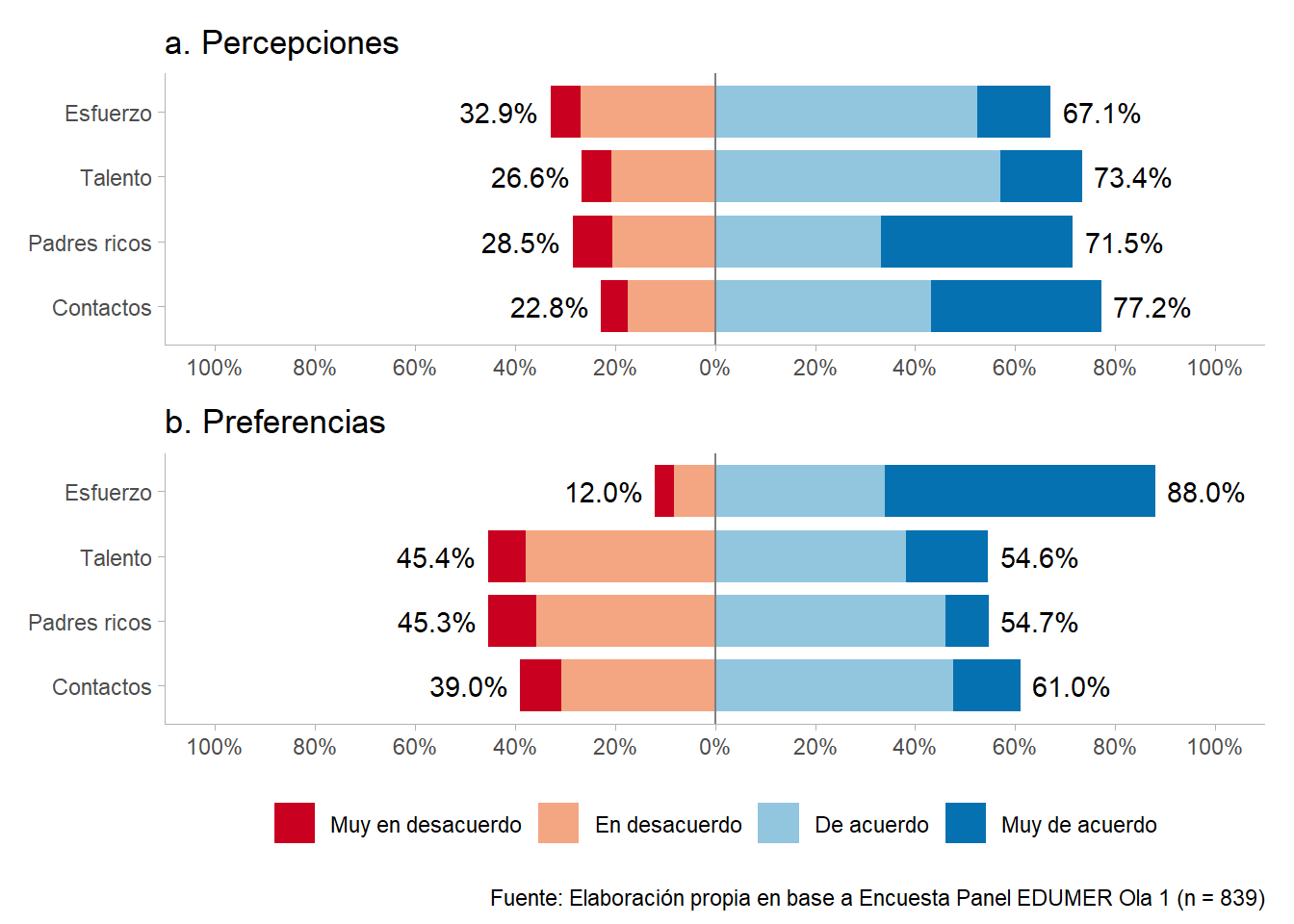
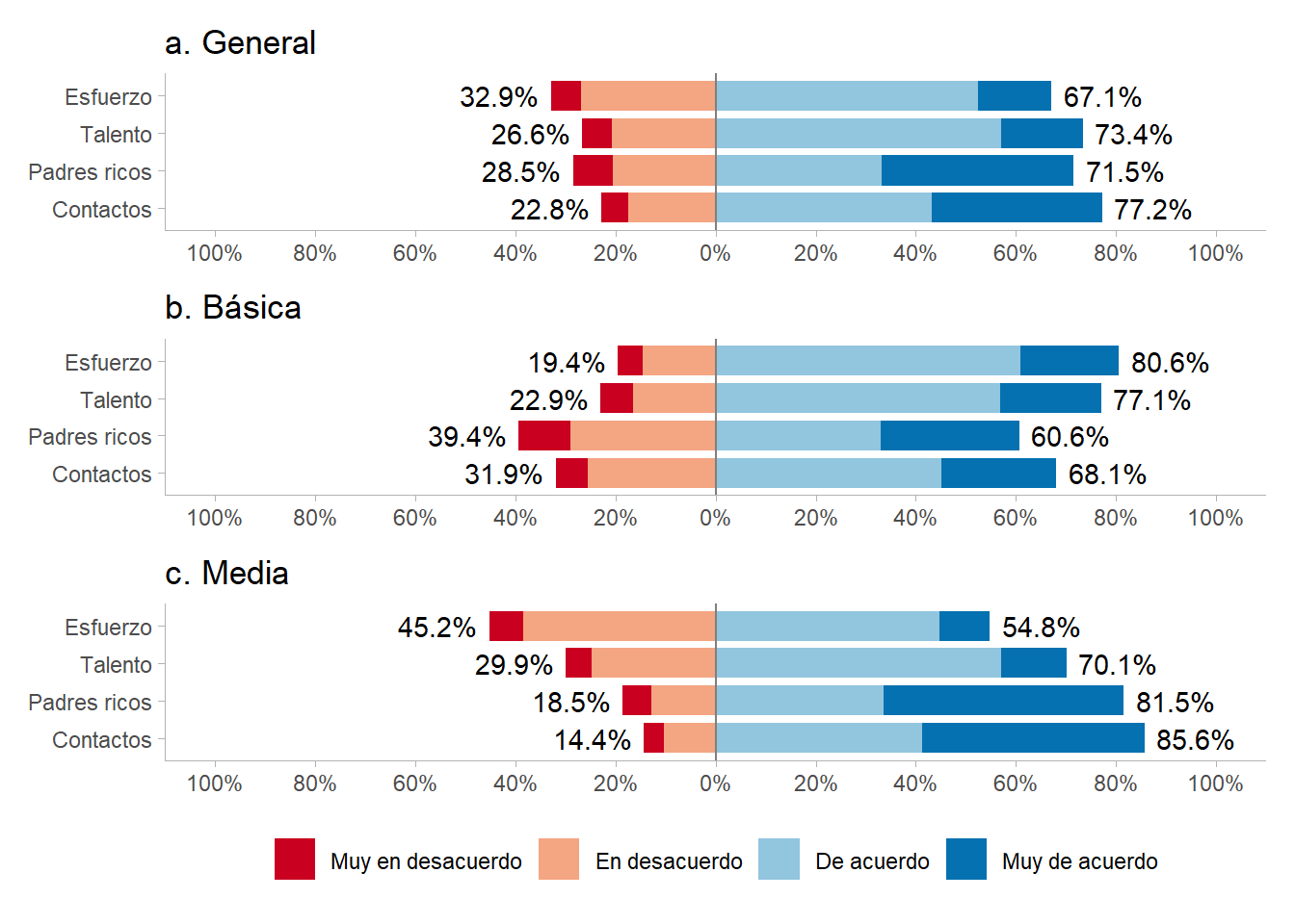
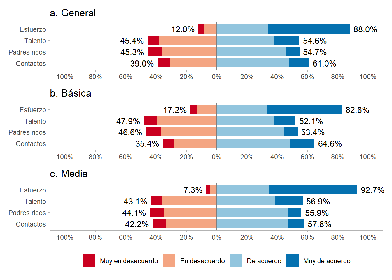
3.1 Descriptives
general <- db1 %>%
  skim() %>%
  yank("numeric") %>%
  as_tibble() %>%
  mutate(range = paste0("(",p0,"-",p100,")")) %>%
  mutate_if(.predicate = is.numeric, .funs = ~ round(.,2)) %>%
  select("Variable" = skim_variable,"Mean"= mean, "SD"=sd, "Range" = range, "Histogram"=hist)

general %>%
kableExtra::kable(format = "markdown")| Variable | Mean | SD | Range | Histogram |
|---|---|---|---|---|
| perc_effort | 2.76 | 0.77 | (1-4) | ▁▅▁▇▂ |
| perc_talent | 2.84 | 0.76 | (1-4) | ▁▃▁▇▂ |
| perc_rich_parents | 3.02 | 0.95 | (1-4) | ▂▅▁▇▇ |
| perc_contact | 3.06 | 0.85 | (1-4) | ▁▃▁▇▆ |
| pref_effort | 3.38 | 0.79 | (1-4) | ▁▁▁▅▇ |
| pref_talent | 2.63 | 0.84 | (1-4) | ▂▇▁▇▃ |
| pref_rich_parents | 2.54 | 0.78 | (1-4) | ▂▆▁▇▂ |
| pref_contact | 2.66 | 0.81 | (1-4) | ▂▅▁▇▂ |
| just_educ | 2.28 | 0.89 | (1-4) | ▅▇▁▆▂ |
| just_health | 2.00 | 0.94 | (1-4) | ▇▇▁▅▂ |
| just_pension | 2.05 | 0.87 | (1-4) | ▆▇▁▅▁ |
| mjp | 2.11 | 0.75 | (1-4) | ▆▇▆▃▁ |
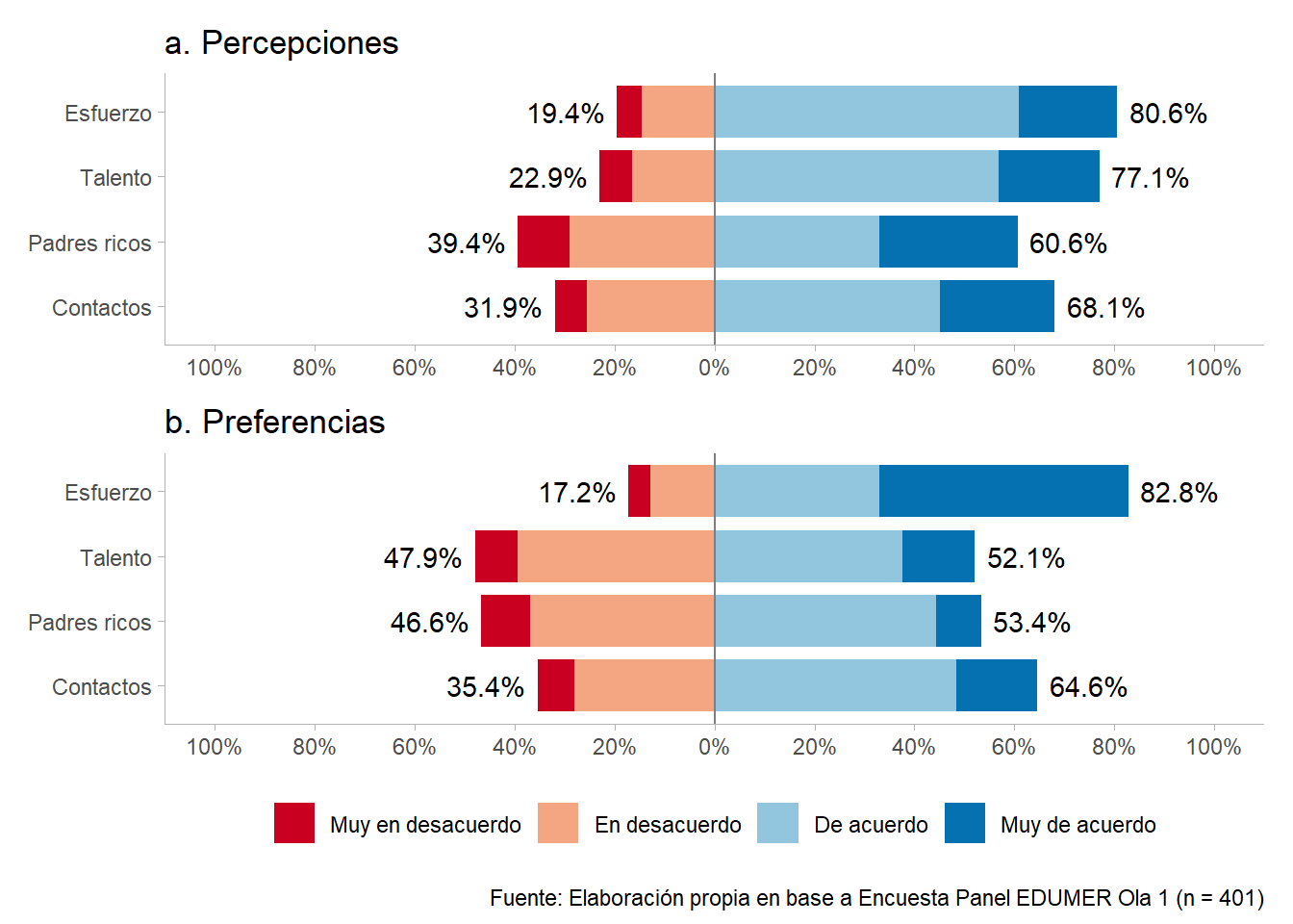
basica <- db1 %>%
  filter(curse_level == "Básica") %>%
  skim() %>%
  yank("numeric") %>%
  as_tibble() %>%
  mutate(range = paste0("(",p0,"-",p100,")")) %>%
  mutate_if(.predicate = is.numeric, .funs = ~ round(.,2)) %>%
  select("Variable" = skim_variable,"Mean"= mean, "SD"=sd, "Range" = range, "Histogram"=hist)

basica %>%
kableExtra::kable(format = "markdown")| Variable | Mean | SD | Range | Histogram |
|---|---|---|---|---|
| perc_effort | 2.95 | 0.74 | (1-4) | ▁▂▁▇▂ |
| perc_talent | 2.91 | 0.79 | (1-4) | ▁▂▁▇▃ |
| perc_rich_parents | 2.78 | 0.97 | (1-4) | ▂▇▁▇▇ |
| perc_contact | 2.85 | 0.85 | (1-4) | ▁▅▁▇▅ |
| pref_effort | 3.28 | 0.85 | (1-4) | ▁▂▁▅▇ |
| pref_talent | 2.58 | 0.84 | (1-4) | ▂▇▁▇▃ |
| pref_rich_parents | 2.53 | 0.79 | (1-4) | ▂▆▁▇▂ |
| pref_contact | 2.73 | 0.82 | (1-4) | ▁▅▁▇▃ |
| just_educ | 2.39 | 0.92 | (1-4) | ▅▇▁▇▂ |
| just_health | 2.19 | 0.97 | (1-4) | ▇▇▁▆▂ |
| just_pension | 2.17 | 0.90 | (1-4) | ▅▇▁▆▂ |
| mjp | 2.25 | 0.78 | (1-4) | ▆▇▇▅▂ |
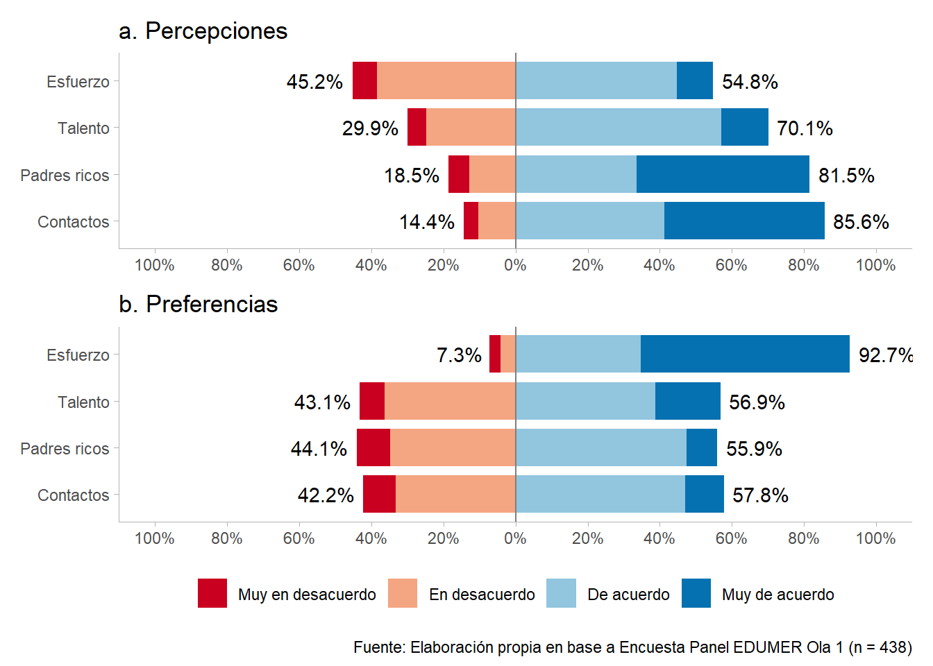
media <- db1 %>%
  filter(curse_level == "Media") %>%
  skim() %>%
  yank("numeric") %>%
  as_tibble() %>%
  mutate(range = paste0("(",p0,"-",p100,")")) %>%
  mutate_if(.predicate = is.numeric, .funs = ~ round(.,2)) %>%
  select("Variable" = skim_variable,"Mean"= mean, "SD"=sd, "Range" = range, "Histogram"=hist)

media %>%
kableExtra::kable(format = "markdown")| Variable | Mean | SD | Range | Histogram |
|---|---|---|---|---|
| perc_effort | 2.58 | 0.76 | (1-4) | ▁▇▁▇▂ |
| perc_talent | 2.78 | 0.73 | (1-4) | ▁▃▁▇▂ |
| perc_rich_parents | 3.24 | 0.88 | (1-4) | ▁▂▁▆▇ |
| perc_contact | 3.26 | 0.80 | (1-4) | ▁▂▁▇▇ |
| pref_effort | 3.47 | 0.72 | (1-4) | ▁▁▁▅▇ |
| pref_talent | 2.68 | 0.85 | (1-4) | ▂▇▁▇▃ |
| pref_rich_parents | 2.55 | 0.78 | (1-4) | ▂▆▁▇▂ |
| pref_contact | 2.59 | 0.80 | (1-4) | ▂▆▁▇▂ |
| just_educ | 2.17 | 0.86 | (1-4) | ▅▇▁▅▁ |
| just_health | 1.82 | 0.88 | (1-4) | ▇▆▁▃▁ |
| just_pension | 1.94 | 0.83 | (1-4) | ▇▇▁▅▁ |
| mjp | 1.98 | 0.69 | (1-4) | ▆▇▅▂▁ |
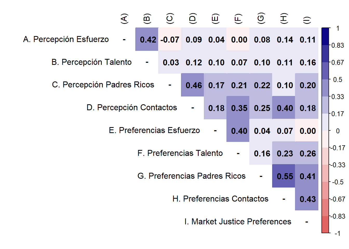
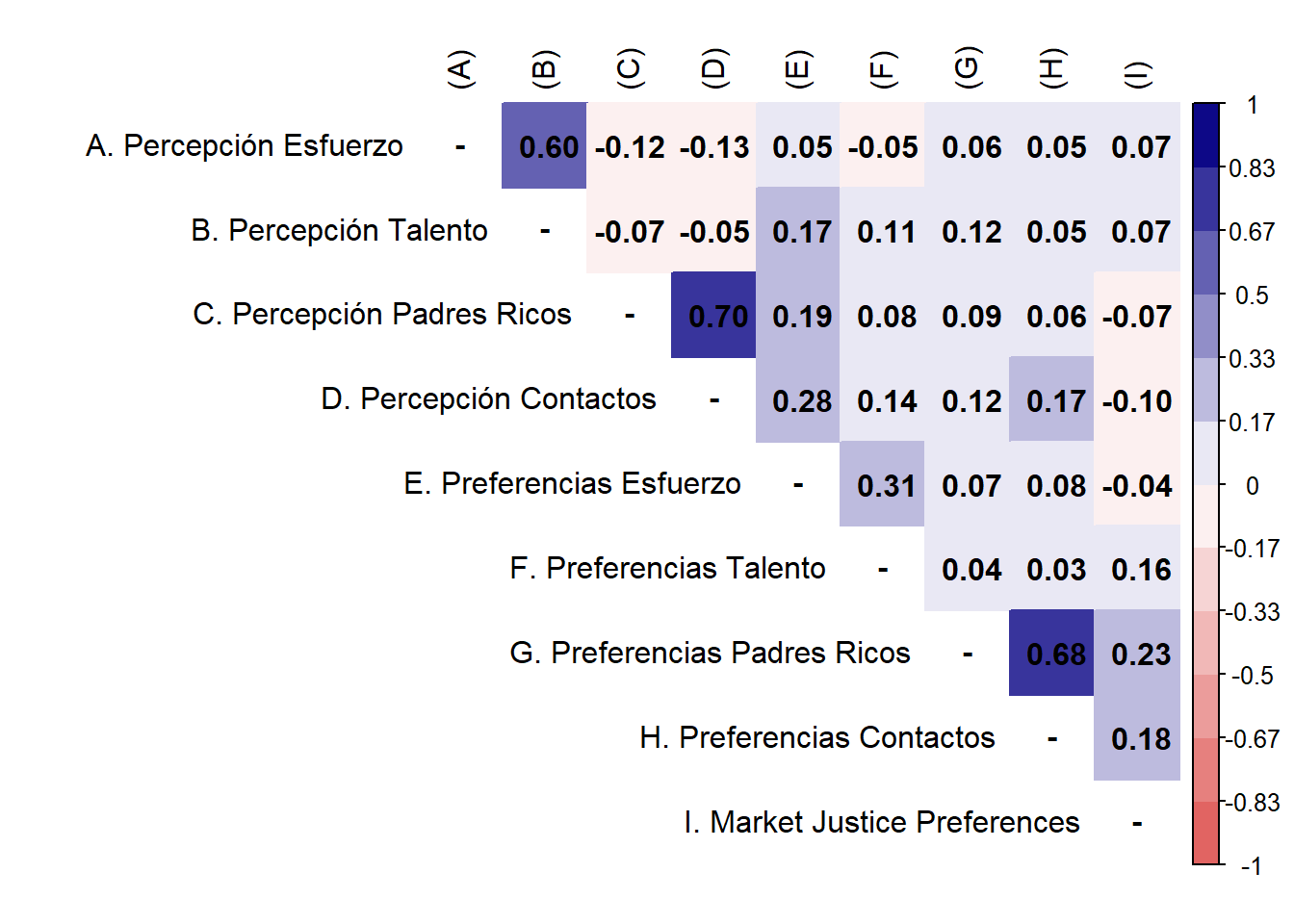
3.2 Bivariates
3.3 Confirmatory factor analysis
model_cfa <- '
  perc_merit = ~ perc_effort + perc_talent
  perc_nmerit = ~ perc_rich_parents + perc_contact
  pref_merit = ~ pref_effort + pref_talent
  pref_nmerit = ~ pref_rich_parents + pref_contact
  '
3.4 Models by cohort
mgeneral_cfa <- cfa(model = model_cfa,
                   data = db1,
                   estimator = "DWLS",
                   ordered = T,
                   std.lv = F)

mbasica_cfa <- cfa(model = model_cfa,
                   data = subset(db1, curse_level == "Básica"),
                   estimator = "DWLS",
                   ordered = T,
                   std.lv = F)

mmedia_cfa <- cfa(model = model_cfa,
                  data = subset(db1, curse_level == "Media"),
                  estimator = "DWLS",
                  ordered = T,
                  std.lv = F)
This section describes the results of the confirmatory factor analysis estimation. The model estimated four latent factors, which were presented in the variables section: meritocratic perceptions, non-meritocratic perceptions, meritocratic preferences, and non-meritocratic preferences.
| Factor | Indicator | Loadings Básica | Loadings Media |
|---|---|---|---|
| perc_merit | perc_effort | 0.56 | 0.66 |
| perc_merit | perc_talent | 0.76 | 0.92 |
| perc_nmerit | perc_rich_parents | 0.48 | 0.69 |
| perc_nmerit | perc_contact | 0.94 | 1.01 |
| pref_merit | pref_effort | 0.45 | 0.83 |
| pref_merit | pref_talent | 0.88 | 0.37 |
| pref_nmerit | pref_rich_parents | 0.64 | 0.85 |
| pref_nmerit | pref_contact | 0.86 | 0.81 |
Based on the four latent factor model, the analysis consisted of estimating and comparing the fit indicators of three models: a general model, one for elementary school students, and another for high school students.
Table 4 shows the standardized factor loadings, estimated with DWLS, for the models for primary and secondary education. The loadings vary greatly depending on the indicator. In the meritocratic preferences factor, the factor loading for preference for effort in the primary model is 0.45, while in the secondary model it is 0.83. This means that the factor in the secondary model is much stronger, explaining almost twice as much of the indicator as in the primary model. Within the same factor is the indicator of preferences for talent, which in primary education has a factor loading of 0.88, suffering a considerable decline in the secondary education model, scoring 0.37. In this sense, the item of preference for talent poorly measures the factor of meritocratic preferences in the secondary education model, but not in the primary education model. A general case in both models is the high factor loading of the perception of contacts item in the non-meritocratic perceptions factor, with 0.94 in the basic model and 1.01 in the average model. It should be noted that this table reflects standardized loadings, so this loading in the average model is an anomalous result, which could cause problems in subsequent estimates.
| chisq | df | pvalue | cfi | tli | rmsea | srmr | |
|---|---|---|---|---|---|---|---|
| Completo | 39.183 | 14 | 0.000 | 0.989 | 0.979 | 0.046 | 0.038 |
| Básica | 17.430 | 14 | 0.234 | 0.996 | 0.992 | 0.025 | 0.036 |
| Media | 11.779 | 14 | 0.624 | 1.000 | 1.003 | 0.000 | 0.029 |
Table 5 shows the fit indices for each of the three models. All models achieved a non-significant chi-square, which could be expected given their sensitivity to large samples, such as those used in this study. It is noteworthy that, for the secondary education model, most indicators have values that are close to perfect (CFI=1.0, TLI=1.003, RMSEA=0, \(\chi^2\)(df=14)=11.779). However, the results of this model could be overfitting, so they should be interpreted with caution. The model for primary education is the one with the best fit (CFI=0.996, RMSEA=0.025, \(\chi^2\)(df=14)=17. 430), while the model that addresses both school levels has comparatively lower fit measures, but acceptable within conventional criteria (CFI=0.989, RMSEA=0.046, \(\chi^2\)(df=14)=39.183).
| Model | χ² (df) | CFI | RMSEA (90% CI) | Δ χ² (Δ df) | Δ CFI | Δ RMSEA | Decision |
|---|---|---|---|---|---|---|---|
| Configural | 36.82 (28) | 0.991 | 0.027 \n (0-0.049) | ||||
| Metric | 49.54 (32) | 0.982 | 0.036 \n (0.013-0.055) | 12.721 (4) * | -0.009 | 0.009 | Reject |
| Strong | 79.27 (36) | 0.955 | 0.054 \n (0.038-0.07) | 29.728 (4) *** | -0.027 | 0.017 | Reject |
| Strict | 145.3 (44) | 0.894 | 0.074 \n (0.061-0.088) | 66.025 (8) *** | -0.061 | 0.021 | Reject |
| Note: N = 839; Group 1, n = 401; Group 2, n = 438 |
The results of the different invariance models are displayed at Table 6. The configurational model has good fit indices (CFI = 0.001, RMSEA = 0.027), although this is only the basis for the upcoming invariance estimates. Looking at the metric model, it appears that when factor loadings are restricted to equality, the four-factor latent model is not equivalent across the different cohorts in the study, despite meeting the \(\Delta\)CFI criteria, which mean rejecting the model if > 0. 01, as well as the \(\Delta\)RMSEA being below the cutoff point (\(\Delta\)RMSEA > 0.015 is rejected). The problem is the p-value < 0.05, which indicates that there are significant differences between the two groups. In this sense, as the following models restrict more parameters, their fit becomes more complex, which is reflected in the fact that none of the following models are accepted. This means that the measurement of the meritocracy scale for students varies depending on the cohort.
3.5 Others